Model comparison
To evaluate these competing hypotheses, we can examine their empirical predictions. Using the same model comparison techniques from adjectives, we compute expected log pointwise predictive densities (ELPDs).
Posterior predictive checks
First, let’s visualize how well each model captures the distribution of responses:
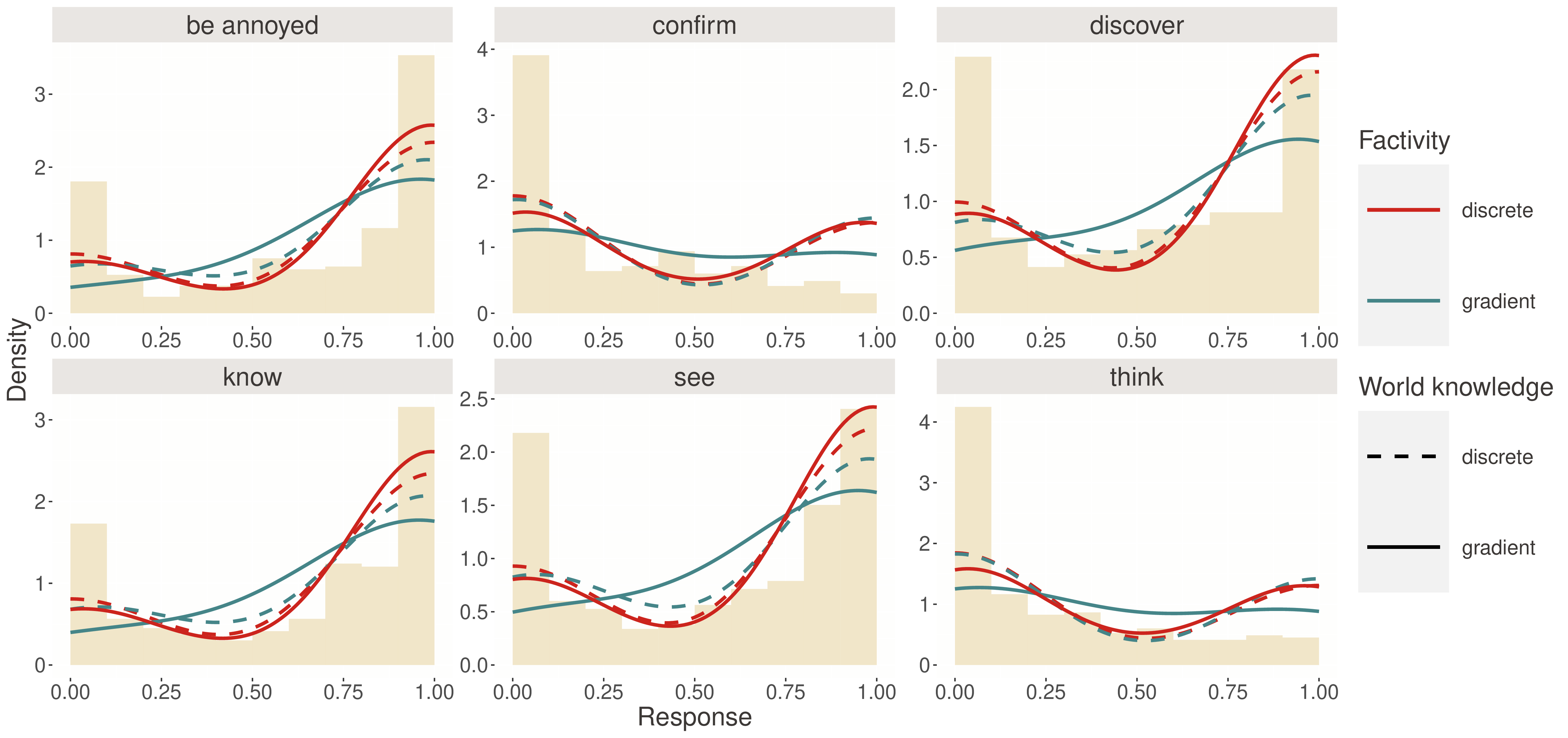
Figure 1 reveals striking differences between the models:
- Discrete-factivity (top left): Captures the characteristic dips in response frequency mid-scale—reflecting its mixture of factive (response ≈ 1) and non-factive (response varies) interpretations
- Wholly-gradient (bottom left): Produces smoother, unimodal distributions, unable to capture the multi-modal patterns in the data
- Wholly-discrete (top right): Forces responses to extremes, missing the intermediate values
- Discrete-world (bottom right): Shows some bimodality but in the wrong direction
The discrete-factivity model’s ability to capture the non-monotonic response patterns is particularly clear for predicates like announce and confirm, where responses cluster both near 1 (factive interpretation) and at intermediate values (non-factive interpretation modulated by world knowledge).
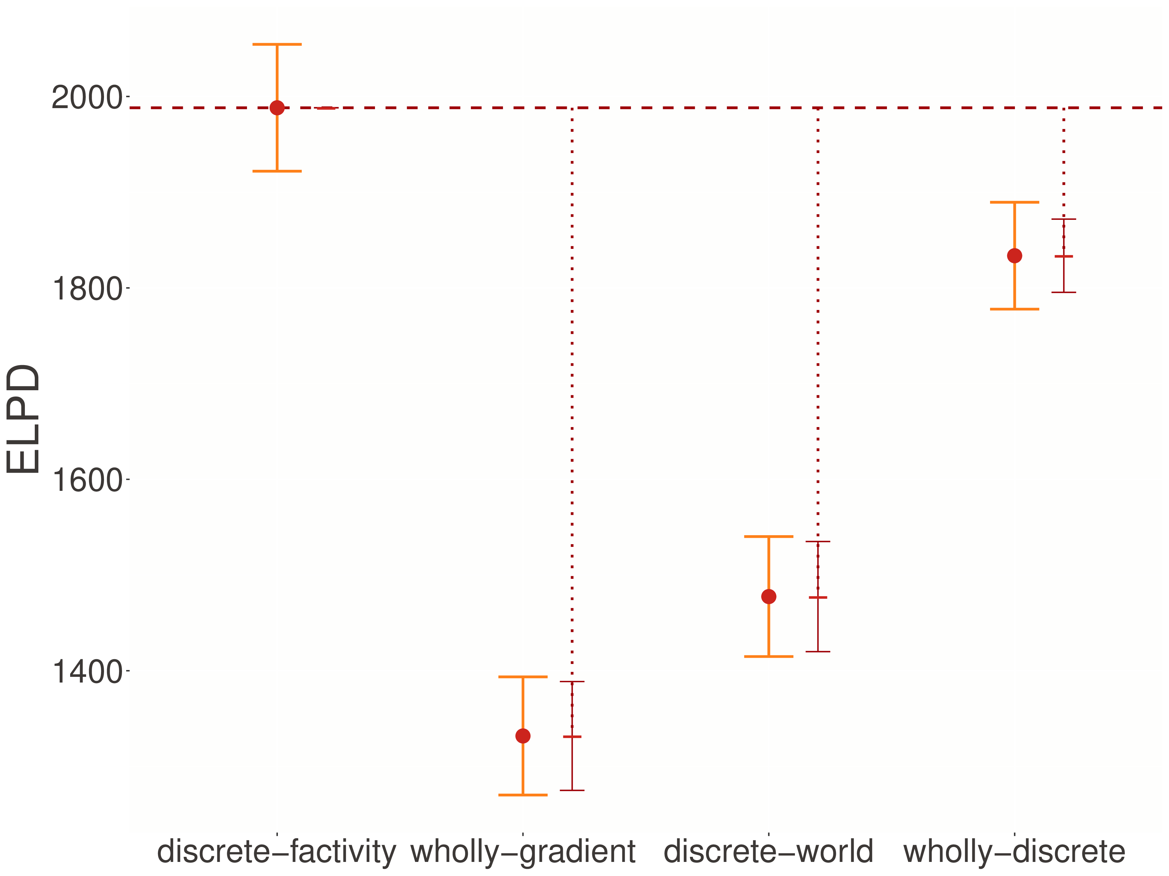
Quantitative comparison
Looking at the expected log pointwise predictive densities reveals a clear winner. The discrete-factivity model substantially outperforms all alternatives across the board. Compared to the wholly-gradient model, it achieves a ΔELPD of 834.5 ± 55.4—a massive improvement in predictive accuracy. The advantages over discrete-world (ΔELPD = 766.1 ± 53.8) and wholly-discrete (ΔELPD = 295.1 ± 34.8) models are similarly impressive. These differences are not just statistically significant but practically large, indicating that the discrete-factivity model provides a dramatically better account of the data.